|
SLJ Test
1.0
System Latency Jitter Test
|
|
SLJ Test
1.0
System Latency Jitter Test
|
bin/<Platform>/sljtest cmd window and run sljtext.exe in that. cd src; make; ./sljtest Ultra Messaging customers use our software to build complicated systems that often process millions of messages per second. Common goals are low latency and high throughput, but many customers also value freedom from latency jitter. A system with no latency jitter would show exactly the same latency for every message passing through it. Consistency is the hallmark of low-jitter systems.
It's hard to be consistent in doing repetitive work when you're being interrupted all the time. For humans, consistency in performing a repeated task requires freedom from interruptions.
Roughly the same idea applies to computer systems. SLJ Test measures the ability of a system to provide a CPU core that is able to consistently execute a repetitive task. The emphasis is not on the average time taken to do a task but rather on the variance in time between repetitions of the task.
We will define system latency jitter more thoroughly below, but for now we can think of it as the jitter measured by an application that introduces no jitter of its own. System latency jitter will be present in any application run by the system. It represents the lower bound for jitter that might be expected of any application running on the system.
SLJ Test measures system latency jitter and provides a simple but effective visualization of it for analysis.
Running a system latency jitter benchmark under different conditions can provide insight into the causes of system latency jitter. Here are some test ideas:
The design of SLJ Test was motivated by goals, but bounded by constraints.
Two key design goals drove the development of SLJ Test:
The above goals had to be met within several design constraints.
The CPU's Time Stamp Counter (TSC) is useful for measuring how long tasks take, especially when very short times are involved. It's usually counting at a rate of 3 or 4 billion counts per second. That gives it a resolution of 333 to 250 picoseconds.
Elapsed ticks can be measured by reading the TSC before and after doing a task, then subtracting the timestamps. This gives the number of ticks taken by the task, plus the time taken to read the TSC once.
When elapsed ticks for an interval are known, the elapsed time in seconds can be computed by dividing elapsed ticks by the CPU frequency in Hertz.
When elapsed time for an interval is known, CPU frequency in Hertz can be computed by dividing the elapsed ticks by the elapsed time.
If a task is repeated many times while measuring elapsed ticks, there will undoubtedly be some variation (jitter) in the number of ticks taken to do the task, even though the work should be the same each time for tasks with no conditional logic.
Jitter is most apparent when we measure the elapsed time taken to do quick tasks. The limiting case is to measure the time needed to just read the TSC. Measuring the delta between two adjacent readings of the TSC does this. It is equivalent to measuring the elapsed time taken by a null task, plus the time to read the TSC.
We want to avoid conditional logic since it may cause jitter by varying CPU cache hit rates. We want to quickly take as many timestamp pairs as possible to maximize jitter detection opportunities. Both these goals are met by using manual loop unwinding to collect the timestamps. Analysis work on the collected timestamps is never done while collecting, but only after completion of the unwound loop.
It's true that each repeated test would run at the minimum elapsed time if there were no jitter. Any test repetition that takes longer than the minimum was delayed by waiting for some system resource. It had to wait because there was contention for a resource that was already in use elsewhere and could not be shared. Examples of shared resources might be data paths on the CPU chip, hyperthreaded execution units, shared caches, memory busses, CPU cores, kernel data structures and critical sections. So it's correct but simplistic to say that all jitter comes from contention.
We can make better progress at reducing jitter if we identify discrete sources of jitter and categorize them for discussion and measurement.
The CPU scheduler in the OS can be a source of jitter if a thread is moved between CPU cores since cache misses in the new core will initially slow execution compared to the old core. Virtual machine hypervisors may prevent a thread from holding the attention of a CPU core indefinitely. Even things at the CPU hardware level like shared cache contention and hyperthreading can add jitter.
Jitter in elapsed time measurements for doing identical tasks is also a measure of things distracting a CPU core from running a thread. Some runs of a task may take longer than others because a CPU core is not able to finish the task without first doing additional work. Hardware interrupts are one possible source of such additional work, but it's best to think of interruptions more broadly. Anything that keeps a CPU core from executing at full speed is a distraction that hurts performance and adds jitter.
Since jitter sources exist at many layers of a system, we can envision a stack of jitter sources by layer as shown below:
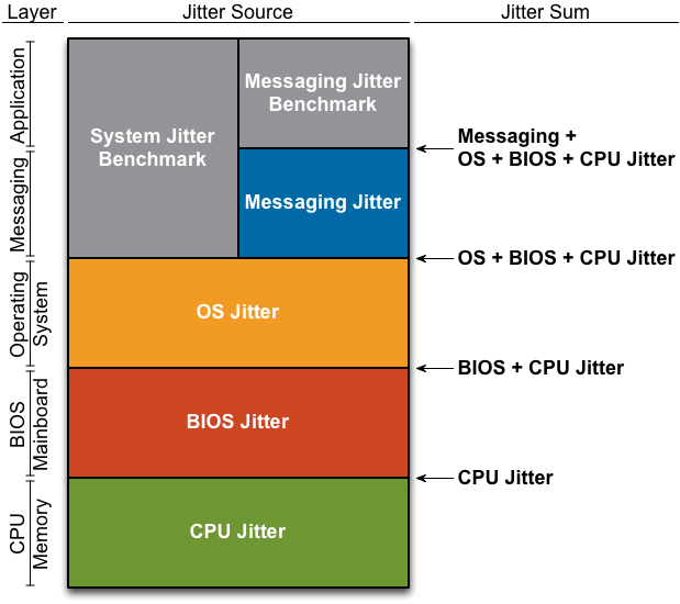
Note that jitter measurements from lower layers propagate to higher layers.
This code aims to measure system latency jitter so that a system can be tuned to minimize it. Reducing jitter in elapsed time measurements made with the TSC minimizes jitter throughout the system. Reading the TSC value is a very low-level operation. It is independent of higher-level languages and libraries like Ultra Messaging.
We define system latency jitter as the jitter measured at the lowest-possible level at which messaging or application software can be written. Applications are the likely source of any jitter measured in excess of the system latency jitter.
SLJ Test uses no network I/O, no messaging library, no memory-managed language, or abstraction layers. It's measuring jitter as close to the machine hardware as we know how to get with C and in-line assembler. Said differently, jitter measured by SLJ Test is coming from server hardware, BIOS, CPU, VM, and OS sources.
Applications doing repetitive tasks may introduce their own jitter by slightly varying the task. Conditional execution in the form of branches and loops is an obvious source of jitter because of cache misses and other effects. Even when code paths appear to be free from branches and loops, jitter can be caused by library calls like malloc() and free() that necessarily contain their own conditional code paths. We categorize all such jitter as application jitter.
Adding networking, messaging libraries, memory-managed language wrappers, and/or abstraction layers will only magnify the effects of system latency jitter. One microsecond of jitter on each step of a 1000-step task can turn into one millisecond of jitter for the whole task.
Note that we use the term "jitter" here in the general sense meaning variation from an expected norm. The system latency jitter discussed here is just one component of the latency variation observed in application-level tests like repeated message round-trip time tests. The standard deviation of latency measured in message round-trip times is often loosely called "jitter," but we are making a distinction here between that and system latency jitter. System latency jitter is that component that can never be removed from an application jitter measurement because it is present in all applications running on the system.
Even a short system latency jitter test produces many millions of data points, so a concise visualization of the data is required to quickly interpret the results. Specifically, a good visualization of the data would allow quick and meaningful comparisons with other test runs.
A histogram is the natural choice for visualizing system latency jitter test data. Histograms are commonly used in applications like displaying the variance in adult height among a population. However, inherent differences in system latency jitter data and display constraints suggest we make some changes from common histograms. Specifically, we use non-uniform bin spacing, logarithmic value display, and rotated axes. Details are presented in following sections.
Although many natural processes follow a normal distribution, the elapsed times measured in system latency jitter tests are not expected to follow a normal distribution. One reason is that there is a hard lower bound on the time required to read the TSC so we shouldn't expect a symmetric or uniform distribution around the mean. Indeed in most cases, the mean and at least one mode are quite close to the lower bound with a very long tail of outliers. Another reason is that the different processes that introduce jitter often produce multimodal distributions.
We often see two or more closely-spaced modes near the lower bound and then several more widely-spaced modes that are perhaps orders of magnitude greater. Conventional linear histogram bin spacing would not visualize this data well. Small numbers of bins would combine nearby modes that have distinct causes. Large numbers of bins leave many bins empty and make it difficult to see patterns.
A high-resolution display might be able to distinctly show both closely- and widely-spaced modes with consistent scaling, but it's hard to write portable code for high-resolution displays.
A graph of the cumulative percentage of all samples always rises from 0 to 100% as we move across the histogram bins. With system latency jitter data, we often see the cumulative percentage rise quickly from 0 to >90% in just a few bins, but then rise much more slowly after that. Thus a graph of the cumulative percentage often shows a knee range where the growth per bin slows.
We make it easier for modes to be seen by using two different bin spacings in the same histogram. The number of bins in the histogram is divided into two halves. The lower half of the bins are lineraly spaced while the upper half are exponentially spaced. This provides detail near the lower bound where modes are closely spaced, while preserving the range needed to show modes that occur 5 or more orders of magnitude above the mean. For linguistic convenience, the bins in the lower half of the histogram are said to be "below the knee," while those in the upper half are above.
The hard lower bound mentioned above means that bins near 0 will likely be empty. We define a minimum expected value that improves the resolution below the knee. Any values below the expected minimum are accumulated in the first bin.
Command line options allow setting the number of bins, the knee value, and a minimum value which is the lower bound of the first bin. Here is an example for 20 histogram bins with a minimum value of 10% of the knee value:
 Bin            Range
 0              min +  0- 10% * (knee-min)
 1              min + 10- 20% * (knee-min)
 2              min + 20- 30% * (knee-min)
 3              min + 30- 40% * (knee-min)
 4              min + 40- 50% * (knee-min)
 5              min + 50- 60% * (knee-min)
 6              min + 60- 70% * (knee-min)
 7              min + 70- 80% * (knee-min)
 8              min + 80- 90% * (knee-min)
 9              min + 90-100% * (knee-min)
 -              --------------------------
 10                       1-2 * knee
 11                      2-10 * knee
 12                     10-20 * knee
 13                    20-100 * knee
 14                   100-200 * knee
 15                  200-1000 * knee
 16                 1000-2000 * knee
 17                2000-10000 * knee
 18               10000-20000 * knee
 19              20000-100000 * knee
Default values produce output that is 28 lines by no more than 80 characters. This small space contains areas with many statistics and a compact visualization of system latency jitter.
The following figure gives a quick overview of the 5 output areas while following sections give detail on each.
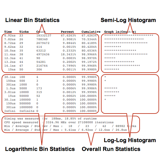
The histogram is displayed rotated 90 degrees clockwise from a conventional display to keep the code portable across operating systems and avoid the requirement for a high-resolution graphical display. The histogram bins are separated by elapsed time and are displayed vertically one bin per line instead of the more conventional horizontal display. The count of the samples in each bin are displayed horizontally instead of the more conventional vertical display.
Note that the number of counts per bin is displayed on a logarithmic scale so that it will fit on low-resolution screens. The magnitude (width) of all bins is scaled so that the bin with the largest count uses the full line width (default 80).
The first half of the bins below the knee setting are linearly spaced in the hope of catching the mode, the average, and the vast majority of the samples. The second half of the bins are spaced roughly by half orders of magnitude so that every pair of bins represents one order of magnitude.
So the top-half (left-half) of the histogram is a semi-log plot while the bottom-half (right-half) is a log-log plot.
Each line of output contains statistics for the associated histogram bin and a visualization of the data. Column values are given in the table below.
| Column | Contents |
|---|---|
| Time | The upper bound of this bin in terms of elapsed time between adjacent reads of the TSC. |
| Ticks | The same as above, but in ticks of the TSC. |
| Count | A count of the number of deltas falling into this bin (only seen without -s flag). |
| Sum | The sum of deltas falling into this bin (only seen with -s flag). |
| Percent | The percentage of all samples in this bin. |
| Cumulative | The cumulative percentage of all samples in this bin and lower. |
| Graph | A graph of the Count column. |
If you want to see more detail in the histogram and have a window with many rows, try increasing the number of bins. Or try increasing the output line width if you have a window with more than 80 columns.
By default, the per-bin statistics and histogram count the deltas that fall into each histogram bin. This weights large and small deltas equally, which can be undesirable if trying to measure the total system latency jitter. The -s flag can be added to the command line to instead report the sum of the deltas that fall into each histogram bin.
After per-bin statistics and histogram lines, there is a section of statistics for the overall test run. While the histogram is useful for characterizing a system's latency jitter and tuning, the overall statistics may be more useful for making benchmark comparisons between systems. In particular, the maximum and standard deviation in units of time are probably the two most important numbers for most Ultra Messaging customers.
Design goals and constraints drove the decision to combine data collection and visualization into a single step. This creates a bit of a chicken-and-egg problem because minimum and knee values must be set before data collection yet the optimal values cannot be known until after data collection and often visualization. The default minimum and knee values may be good enough for a quick analysis, but tuning these values away from the defaults often provides sharper insight.
There are heuristics built into SLJ Test that check the minimum and knee values for reasonability after data collection. You'll see this recommendation if the minimum data sample is less that 80% of the configured expected minimum.
Recommend min setting of x ticks
Where x is 80% of the minimum data sample seen.
Similarly you'll see this recommendation if the cumulative sample count at the middle histogram bin is less than 90% the total samples.
Recommend increasing knee setting from x ticks
Where x is the configured knee value.
Finally you'll see this recommendation if the cumulative sample count at the middle histogram bin is greater than 99% of the total samples.
Recommend decreasing knee setting from x ticks
Where x is the configured knee value.
An outlier is defined as any TSC delta greater than the knee. The -f option names a file where outliers will be written. The format is x, y where x is the time of the outlier in ms relative to the start of the test and y is the size of the outlier in us. Note the different units between axes.
The expectation is that you'll give this data to the graphing software of your choice and request an x y scatter plot. Visual analysis of the plot may help you spot any periodic patterns in the jitter. The period may give you clues to the source of the jitter.
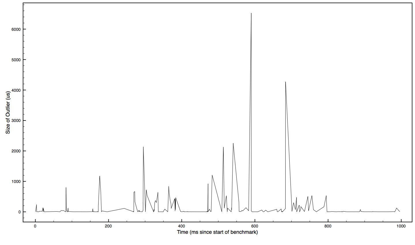
Better yet, do an FFT on the data to move it from the time domain to the frequency domain.
Note that x may not be near zero if the outlier buffer wraps around. If you're worried about the outlier buffer wrapping around, my advice is to increase the knee to classify fewer deltas as outliers rather than making the buffer bigger. The default size is probably big enough for you to spot any periodic patterns.
 -b bins        Set the number of Bins in the histogram (20)
 -f outfile     Name of file for outlier data to be written (no file written)
 -h             Print Help
 -k knee        Set the histogram Knee value in TSC ticks (50)
 -m min         Set the Minimum expected value in TSC ticks (10)
 -o outbuf      Size of outlier buffer in outliers (10000)
 -p pause       Pause msecs just before starting jitter test loop (0)
 -r runtime     Run jitter testing loops until seconds pass (1)
 -s             Sum deltas falling into each bin (instead of just counting deltas falling into bin)
 -w width       Output line Width in characters (80)
Following sections show data collected on various systems under various conditions with comments.
This output came from a server in our lab that had been tuned for low jitter.
Time    Ticks    Count        Percent    Cumulative  Graph ln(Count-e)
10.7ns  32       0             0.0000%    0.0000%
11.4ns  34       0             0.0000%    0.0000%
  12ns  36       6997631      42.0733%   42.0733%    *************************
12.7ns  38       0             0.0000%   42.0733%
13.4ns  40       0             0.0000%   42.0733%
  14ns  42       0             0.0000%   42.0733%
14.7ns  44       0             0.0000%   42.0733%
15.4ns  46       9634329      57.9265%   99.9998%    **************************
  16ns  48       0             0.0000%   99.9998%
16.7ns  50       0             0.0000%   99.9998%

33.4ns  100      0             0.0000%   99.9998%
 167ns  500      0             0.0000%   99.9998%
 334ns  1000     2             0.0000%   99.9998%    *
1.67us  5000     36            0.0002%  100.0000%    *****
3.34us  10000    2             0.0000%  100.0000%    *
16.7us  50000    0             0.0000%  100.0000%
33.4us  100000   0             0.0000%  100.0000%
 167us  500000   0             0.0000%  100.0000%
 334us  1000000  0             0.0000%  100.0000%
Infini  Infinite 0             0.0000%  100.0000%

Timing was measured for  229ms, 22.91% of runtime
CPU speed measured  : 2992.58 MHz over 16632000 iterations
Min / Average / Std Dev / Max :   36   /   41   /    6   / 6984 ticks
Min / Average / Std Dev / Max :   12ns / 13.7ns / 1.67ns / 2.33us
42% of the samples were in the 12 ns bin and almost 58% were in the 15.4 ns bin. Together, 99.9998% of all samples were in these two bins. There were zero samples in the 4 bins between these two, producing a nice bi-modal histogram. The outlier samples were just 36 out of 16.6 million.
This output came from a busy server in our lab.
Time    Ticks    Count        Percent    Cumulative  Graph ln(Count-e)
6.92ns  23       18332137     67.6263%   67.6263%    **************************
7.82ns  26       788340        2.9081%   70.5344%    *********************
8.72ns  29       2679472       9.8844%   80.4189%    ***********************
9.62ns  32       414           0.0015%   80.4204%    *********
10.5ns  35       63212         0.2332%   80.6536%    *****************
11.4ns  38       4972436      18.3431%   98.9966%    ***********************
12.3ns  41       90            0.0003%   98.9970%    ******
13.2ns  44       54281         0.2002%   99.1972%    ****************
14.1ns  47       216764        0.7996%   99.9968%    *******************
  15ns  50       306           0.0011%   99.9980%    ********

30.1ns  100      4             0.0000%   99.9980%    *
 150ns  500      3             0.0000%   99.9980%    *
 301ns  1000     0             0.0000%   99.9980%
 1.5us  5000     173           0.0006%   99.9986%    *******
3.01us  10000    315           0.0012%   99.9998%    ********
  15us  50000    52            0.0002%  100.0000%    ******
30.1us  100000   1             0.0000%  100.0000%    *
 150us  500000   0             0.0000%  100.0000%
 301us  1000000  0             0.0000%  100.0000%
Infini  Infinite 0             0.0000%  100.0000%

Timing was measured for  188ms, 18.85% of runtime
CPU speed measured  : 3324.96 MHz over 27108000 iterations
Min / Average / Std Dev / Max :   18   /   23   /   42   / 88982 ticks
Min / Average / Std Dev / Max : 5.41ns / 6.92ns / 12.6ns / 26.8us
It shows a much faster average time than the low-jitter server above, but the standard deviation is over 7 times larger while the maximum is over 11 times larger.
Informatica makes the binary and source code for SLJ Test freely available so that our customers can use it to work with their hardware and software vendors to reduce jitter. We pioneered this idea with our mtools software for testing multicast UDP performance. Many customers have used mtools to work with their NIC, driver, OS, and server vendors to improve UDP multicast performance. We hope that this code can be used between our customers and their other vendors to reduce system latency jitter.
Gil Tene of Azul Systems has written jHiccup, a tool for measuring latency jitter in Java JVM runtime systems.
Inspired by David Riddoch of Solarflare
Idea for -s flag to sum deltas into histogram bins instead of just counting them from Erez Strauss
Redistribution and use in source and binary forms, with or without modification, are permitted without restriction. The author will be disappointed if you use this software for making war, mulching babies, or improving systems running competing messaging software.
THE SOFTWARE IS PROVIDED "AS IS" AND INFORMATICA DISCLAIMS ALL WARRANTIES EXPRESS OR IMPLIED, INCLUDING WITHOUT LIMITATION, ANY IMPLIED WARRANTIES OF NON-INFRINGEMENT, MERCHANTABILITY OR FITNESS FOR A PARTICULAR PURPOSE. INFORMATICA DOES NOT WARRANT THAT USE OF THE SOFTWARE WILL BE UNINTERRUPTED OR ERROR-FREE. INFORMATICA SHALL NOT, UNDER ANY CIRCUMSTANCES, BE LIABLE TO LICENSEE FOR LOST PROFITS, CONSEQUENTIAL, INCIDENTAL, SPECIAL OR INDIRECT DAMAGES ARISING OUT OF OR RELATED TO THIS AGREEMENT OR THE TRANSACTIONS CONTEMPLATED HEREUNDER, EVEN IF INFORMATICA HAS BEEN APPRISED OF THE LIKELIHOOD OF SUCH DAMAGES.
 1.8.1.2

